AIPT Section 4.1: CFR – The CFR Algorithm

CFR - The CFR Algorithm

The Counterfactual Regret Minimization (CFR) algorithm was first published in a 2007 paper from the University of Alberta by Martin Zinkevich et al. called “Regret Minimization in Games with Incomplete Information”.

Counterfactual means “relating to or expressing what has not happened or is not the case”. For example, if in reality I didn’t bring an umbrella and got wet in the rain, I could say counterfactually, “If I had brought an umbrella, I wouldn’t have gotten wet.”

Regret we previously touched on in the Game Theory Foundation section. In brief, it’s a way to assign a value to the difference between a made decision and an optimal decision. For example, if you choose to play a slot machine that returns a value of 5 rather than a machine that returns a value of 10, then your regret would be 10-5 = 5.

Minimization refers to minimizing the difference between the made decision and the optimal decision. Playing the slot machine that returns a value of 10 (i.e. the optimal machine) would minimize the regret to 0. Of course this is a very simple example and things aren’t usually that easy.

TLDR Explanation

CFR is a self play algorithm that learns by playing against itself repeatedly. It starts play with a uniform random strategy (each action at each decision point is equally likely) and iterates on these strategies to nudge closer to the game theory optimal Nash equilibrium strategy as the self play continues (the average of all strategies converges to the equilibrium strategy). The Nash equilibrium strategy is a fixed “defensive” strategy that can’t be beaten, but also doesn’t take advantage of opponents.

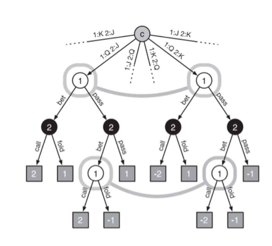
The counterfactual part comes from computing values of actions from a game state based on assuming counterfactually that we play to that game state with probability 1. Therefore only the opponent and chance probabilities to get to this game state are factored into the equation.

The values are called counterfactual values and are computed by multiplying the probability of the opponent and chance playing to a certain state by the probability of playing from that point to the end of the game tree and the value at the end of the game tree.

At each information set in the game tree, the algorithm keeps a counter of regret values for each possible action. The regret means how much better the agent would have done if it had always played that action rather than the average strategy over the mixture of all possible actions. Positive regret means we should have taken that action more and negative regret means we would have done better by not taking that action.

For example, if the agent was playing a game in which it had 5 action options at a certain game state and Action 1 had a value of 3 while the game state average over all 5 actions was 1, then the regret would be 3-1 = 2. This means that Action 1 was better than average and we should favor taking that action more.

The regret is minimized by playing more of the better actions, thus bringing up the average game state value.

The CFR algorithm updates the strategy after each iteration to play in proportion to the regrets, meaning that if an action did well in the past, the agent would be more likely to play it in the future. Note that playing proportionally means we don’t change the strategy too drastically, which could be predictable and exploitable. This also means that strategies that do poorly have a chance to “recover” and be played again.

The final Nash equilibrium strategy is the average strategy over each iteration. This strategy cannot lose in expectation and is considered optimal since it’s theoretically robust and neither player would have incentive to change strategies if both playing an equilibrium. This is what we mean when we say “solve” a poker game.

Detailed Intuitive Explanation

Michael Johanson, one of the authors on the original paper, gave his intuitive explanation of CFR in a post on Quora.

Simplified Counterfactual Value and Regret Computations

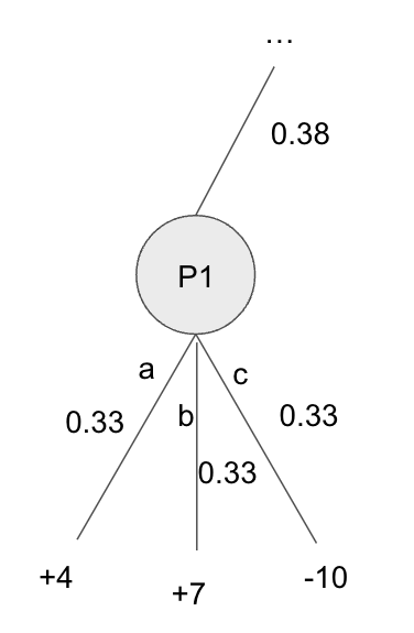
Here we show a very simple game tree showing a Player 1 node at the end of the game. For simplicity, we assume that this is the first iteration of the algorithm so each action is assigned a uniform \(1/3\) probability. \(\sigma_(-i) = 0.38\) is assigned as the probability of chance and Player 2 to play to this node. Player 1’s probability is counterfactually assumed to be \(1\).

Regular expected value: We can compute the regular expected value for each action of P1: \(\text{EV(action)} = P(\text{play from current node to endpoint}) * U(\text{endpoint})\)

\[\text{EV(action)} = \pi^\sigma(h,z) * u_i(z)\]

\(EV(a) = 0.33*(4) = 1.33\) \(EV(b) = 0.33*(7) = 2.33\) \(EV(c) = 0.33*(-10) = -3.33\)

Counterfactual value: The counterfactual value includes the reach probability \(\sigma_(-i) = 0.38\) of the opponent and chance playing to this node.

\(CV()\) v_i(I,a) = \pi^\sigma_{-i}(h)\pi^{\sigma:I\rightarrow a}(h,z)u_i(z) \(\) v

The Algorithm

Due to the constraints of solving imperfect information games with MCTS and the memory limits of solving games with linear programs, CFR was developed as a novel solution. CFR also benefits from being computationally cheap and doesn’t require parameter tuning. It is an iterative Nash equilibrium approximation method that works through the process of repeated self-play between two regret minimizing agents.

CFR is an extension of regret minimization into sequential games, where players play a sequence of actions to reach a terminal game state. Instead of storing and minimizing regret for the exponential number of strategies, CFR stores and minimizes a regret for each information set and its actions, which can be used to form an upper bound on the regret for any deterministic strategy. This means that we must also consider the probabilities of reaching each information set given the players’ strategies, as well as passing forward game state information and probabilities of player actions, and passing backward utility information through the game information states. The algorithm stores a strategy and regret value for each action at each node, such that the space requirement is on the order \(O(|I|)\) , where \(|I|\) is the number of information sets in the game.

CFR is an offline self-play algorithm, as it learns to play by repeatedly playing against itself. It begins with a strategy that is completely uniformly random and adjusts the strategy each iteration using regret matching such that the strategy at each node is proportional to the regrets for each action. The regrets are, as explained previously, measures of how the current strategy would have performed compared to a fixed strategy of always taking one particular action. Positive regret means that we would have done better by taking that action more often and negative regret means that we would have done better by not taking that action at all. The average strategy is then shown to approach a Nash equilibrium in the long run.

In the vanilla CFR algorithm, each iteration involves passing through every node in the extensive form of the game. Each pass evaluates strategies for both players by using regret matching, based on the prior cumulative regrets at each player’s information sets. Before looking at the CFR equations, we will refresh some definitions that were given in previous sections here when they are relevant to the forthcoming equations.

Let \(A\) denote the set of all game actions. We refer to a strategy profile that excludes player \(i\)’s strategy as \(sigma_(-i)\). A history h is a sequence of actions, including chance outcomes, starting from the root of the game. Let \(pi^(sigma)(h)\) be the reach probability of game history \(h\) with strategy profile \(sigma\) and \(pi^sigma(h,z)\) be the reach probability that begins at \(h\) and ends at z.

Let \(Z\) denote the set of all terminal game histories and then we have \(h ⊏ z\) for \(z ∈ Z\) is a nonterminal game history. Let \(u_i(z)\) denote the utility to player \(i\) of terminal history \(z\).

We can now define the counterfactual value at nonterminal history \(h\) as follows: \(v_i(sigma, h) = sum (z in Z),h ⊏ z of pi^sigma_(-i) * pi^sigma(h,z) * u_i(z)\)

This is the expected utility to player \(i\) of reaching nonterminal history \(h\) and taking action a under the counterfactual assumption that player \(i\)takes actions to do so, but otherwise player \(i\) and all other players follow the strategy profile sigma.

The counterfactual value takes a player’s strategy and history and returns a value that is the product of the reach probability of the opponent (and chance) to arrive to that history and the expected value of the player for all possible terminal histories from that point. This is counterfactual because we ignore the probabilities that factually came into player \(i\)’s play to reach position \(h\), which means that he is not biasing his future strategy with his current strategy. This weights the regrets by how often nature (factors outside the player’s control, including chance and opponents) reach this information state. This is intuitive because states that are more frequently played to by opponents are more important to play profitably.

An information set is a group of histories that a player cannot distinguish between. Let \(I\) denote an information set and let \(A(I)\) denote the set of legal actions for information set \(I\). Let \(sigma_(I-->a)\) denote a profile equivalent to sigma, except that action a is always chosen at information set \(I\). The counterfactual regret of not taking action a at history \(h\) is defined as:

\[r(h,a) = v_i(sigma_(i-->a),h) - v_i(sigma, h)\]

This is the difference between the value when always selecting action a at the history node and the value of the history node itself (which will be defined in more detail shortly).

Let \(pi^sigma(I)\) be the probability of reaching information set I through all possible game histories in I. Therefore we have that \(pi^sigma(I) = sum h∈I pi^sigma(h)\). The counterfactual reach probability of information state \(I\), \(p^sigma_(-i)(I)\), is the probability of reaching \(I\) with strategy profile \(sigma\) except that, we treat current player \(I\) actions to reach the state as having probability 1.

The counterfactual regret of not taking action a at information set \(I\) is: \(r(I,a) = sum h∈I r(h,a)\)

This calculation simply includes all histories in the information set.

Let \(t\) and \(T\) denote time steps, where \(t\) is with respect to each fixed information set and is incremented with each visit to an information set. A strategy \(sigma^t_i\) for player \(i\) maps each player \(i\) information set \(I_i\) and legal player \(i\) action \(a∈A(I_i)\) to the probability that the player will choose \(a\) in \(I_i\) at time \(t\). All player strategies together at time \(t\) form a strategy profile \(sigma^t\), to be detailed shortly.

If we define \(r^t_i(I,a)\) as the regret when players use \(sigma_t\) of not taking action \(a\) at information set \(I\) belonging to player \(i\) , then we can define the cumulative counterfactual regret as follows, which is the summation over all time steps:

\[R^T_i(I,a) = sum t=1 to T r^t_i(I,a)\]

In recent years, researchers have redefined the counterfactual value in terms of information sets. This formulation shows the counterfactual value for a particular information set and action, given a player and his strategy:

\[v^sigma_i(I,a) = sum h∈I sum z∈Z: h⊏z u_i(z)pi^sigma_(-i)(z)pi^sigma:I-->a _i(h,z)\]

We see that this is similar to the first equation for the counterfactual value, but has some differences. Because we are now calculating the value for an information set, we must sum over all of the relevant histories. The inner summation adds all possible leaf nodes that can be reached from the current history (same as the original one) and the outer summation adds all histories that are part of the current information set.

From left to right, the three terms on the right hand side represent the main player’s utility at the leaf node \(z\) , the opponent and chance combined reach probability for the leaf node \(z\) , and the reach probability of the main player to go from the current history to the leaf node \(z\) , while always taking action \(a\). The differences between this formulation and that of the original equation will be reconciled with the next equation.

The counterfactual regret of player \(i\) for action \(a\) at information set \(I\) can be written as follows:

\[R^T_i(I,a) = sum t=1,T v^sigma^t _i(I,a) - sum t=1,T sum a'∈A v^sigma^T _i (I,a')sigma^t_i(a'\\|I)\]

This formulation combines the three equations, where one had introduced the cumulative summation, one added all histories in the information set, and one defined the counterfactual regret difference equation. The first part of the difference in the counterfactual regret equation computes this value for the given a value, while the second part computes the expected value of all other a value options at the information set.

The inner summation of this part of the equation is over all non-a strategies and the outer summation is over all times. The first term in the summations computes the counterfactual value for each non-a strategy and the second term multiplies the counterfactual value by the player’s probability of playing that particular strategy at the given information set.

We can show the regret-matching algorithm by first defining the nonnegative counterfactual regret as \(R^T,+ _i (I,a) = max(R^T _i(I,a),0)\) . Now we can use the cumulative regrets to obtain the strategy decision for the next iteration using regret matching:

Case 1 when \(sum a'∈A R^(t-1) _i (I,a'))^+ > 0\) then \(sigma^t _i(a\\|I) = (R^(t-1) _i (i,a))^+ / (sum a'∈A R^(t-1) _i (I,a'))^+)\)

Case 2 otherwise then \(sigma^t _i(a\\|I) = 1/\\| A \\|\)

This regret matching formula calculates the action probabilities for each action at each information set in proportion to the positive cumulative regrets. First we check to see if the cumulative regrets at the previous time step are positive. If not, the strategy is set to be uniformly random, determined by the number of available actions. If it is, then the strategy is the ratio of the cumulative regret of the defined action over the sum of the cumulative regrets of all other actions.

The CFR algorithm works by taking these action probabilities and then producing the next state in the game and computing the utilities of each action recursively. Regrets are computed from the returned values and the value of playing to the current node is then computed and returned. Regrets are updated at the end of each iteration.

Regret Bounds and Convergence Rates

CFR has been shown to eliminate all dominated strategies from its final average strategy solution.

By following regret matching, the following bound, showing that the counterfactual regret at each information set grows sublinearly with the number of iterations, is guaranteed, given that delta = maximum difference in leaf node utilities \((|u_i(z) − u_i(z')| ≤ delta\) for all \(i ∈ N\) and \(z,z' ∈ Z)\) , \(A\) = number of actions, \(T\) = iteration number.

\[R^T _i_infoset(I,a) <= delta * sqrt(\\| A \\| * T)\]

With a specific set of strategy profiles, we can define a player’s overall regret as: \(R^T _i_overall = max sigma_i ∈ sum i (sum t=1 to T u_i(sigma_i, sigma^T _-i)) - sum t=1 to T u_i(sigma)\)

This is the amount of extra utility that player i could have achieved in expectation if he had chosen the best fixed strategy in hindsight. Assuming perfect recall, this can be bounded by the per information set counterfactual regrets of CFR:

\[R^T _i_overall <= sum I∈I_i max a∈A R^T _i_infoset(I,a) <= \\|I_i\\| * delta * sqrt(\\|A\\|*T)\]

The fact that minimizing regret at each information set results in minimizing overall regret is a key insight for why CFR works and since CFR indeed achieves sublinear regret, this means that it is a regret minimizing algorithm.

In a two-player zero-sum game with perfect recall, for \(R^t _i ≤ ε\) for all players, then the average strategy profile is known to be a \(2ε\) Nash equilibrium. We can therefore use the regret minimizing properties of CFR to solve games like poker by computing average strategies as follows:

\[sigmahat(a|I) = [sum t=1,T (sum h∈I pi^sigma^t _i (h)) * sigma^t(a|I)] / [sum t=1,T (sum h∈I pi^sigma^t _i (h)))]\]

where \(sum t=1,T (sum h∈I pi^sigma^t _i (h)))\) is each player’s contribution to the probability of reaching a history in information set \(I\) , and is therefore the weighting term on \(sigma^T _i\).

The strategies are combined such that they select an action at an information set in proportion to that strategy’s probability of playing to reach that information set. We run the CFR algorithm for a sufficient number of iterations in order to reduce the ε sufficiently.

In the end, it is the average strategy profile that converges to Nash equilibrium. The best available guarantees for CFR require ~\(1/ε^2\) iterations over the game tree to reach an \(ε\)-equilibrium, that is, strategies for players such that no player can be exploited by more than \(ε\) by any strategy.

The gradient-based algorithms, which match the optimal number of iterations needed, require only ~\(1/ε\) or ~\(log (1/ε)\) iterations. However, due to effective CFR sampling methods, quick approximate iterations can be used such that sampling CFR is still the preferred solution method.

Why average strategy?

A good intuitive way to think about why at the end of running CFR, the average strategy is the Nash equilibrium rather than the final strategy being Nash equilibrium comes from looking at rock paper scissors.

Suppose that our opponent is playing Rock too much, then CFR moves us towards playing 100% paper (moving towards the best response to their strategy, i.e. the goal of regret minimization). The current strategy can be mixed (and it starts off uniform random), but it gets updated to maximize exploiting opponents and tends to cycle between pure-ish strategies (assuming that we are playing against a real opponent and not using self-play).

So the algorithm moves us to 100% paper and then the opponent might move to 100% scissors and then we move to 100% rock, and so on! While the current strategy is making sharp bounces around the strategy space without stopping at equilibrium, the average strategy cycles in closer and closer to converging at equilibrium, which in rock paper scissors is playing each action a third of the time. Intuitively it makes sense that the average strategy would be more robust than just taking the final strategy, which could be at a strange point that clearly wouldn’t be an equilibrium.

That said, recent research teams have simply used the final strategy after many many iterations and have had good results, which saves a lot of memory and computation since all of the strategies throughout don’t need to be stored and averaged.

Vanilla CFR

Vanilla CFR is the default CFR method where each pass is a full iteration of the game tree. This has been used less ever since the Monte Carlo sampling CFR methods began from Marc Lanctot’s research. Although sampling means a larger number of iterations are needed to reach near equilibrium levels, each iteration is generally much faster and overall calculation time is generally significantly reduced since regrets are updated very quickly, instead of only after every long iteration as is the case with vanilla CFR. Vanilla CFR works by passing forward probabilities and game states and passing back utility values and can solve games as large as about 10^12 game states.

Monte Carlo CFR (MCCFR)

In Monte Carlo CFR, some sampling method is used to sample to terminal state(s) of the game and then updates are applied only to the sample and not the full tree. Other than that, the updates occur the same way as they do in the standard algorithm.

The benefit of Monte Carlo CFR is that it uses sampling to make quicker updates to the game tree, even though these updates may be noisy, in practice they are much faster than the precise and slow updates of the vanilla implementation. Memory requirements remain the same as in vanilla CFR since the same information is being stored.

In practice, this means updating the counterfactual value equation with a \(1/q(z)\) factor to define the probability of sampling a particular terminal history z. Also the summation is defined only for the information set when \(z\) is in the sample and passes through the information set \(I\) on the way to \(z\). It can be shown that the sampled counterfactual values are equivalent in expectation to the vanilla version, meaning that MCCFR also will be guaranteed to converge to a Nash equilibrium.

An issue arises with sampling that when taking the average strategy, all nodes may not have been sampled equal times. This can be addressed in two ways, each of which has its own disadvantages:

1. Optimistic averaging: A counter is placed at each node and updates are weighted by the last time they were seen at this node, which requires extra memory, is only an approximation, and requires a final iteration since some counters will be outdated.
2. Stochastically weighted averaging: Increase the magnitude of each strategy by sampling the strategy profile probability. This is unbiased, but results in large variance.

We touch on two of the most common sampling methods below, called external sampling and chance sampling. Outcome sampling is another method that is the most extreme possible sampling – it samples one action down the whole tree.

External Sampling

External Sampling entails sampling the actions of the opponent and of chance only. This means that these samples are based on how likely the opponent’s plays are to occur, which is sensible, since then regret values corresponding to these plays are updated faster. We go into this in more detail in Section 4.4 regarding Deep CFR, but provide code here in Python for Kuhn Poker and Leduc Poker.

Kuhn External CFR code:

import numpy as np
import random

class Node:
	def __init__(self, num_actions):
		self.regret_sum = np.zeros(num_actions)
		self.strategy = np.zeros(num_actions)
		self.strategy_sum = np.zeros(num_actions)
		self.num_actions = num_actions

	def get_strategy(self):
		normalizing_sum = 0
		for a in range(self.num_actions):
			if self.regret_sum[a] > 0:
				self.strategy[a] = self.regret_sum[a]
			else:
				self.strategy[a] = 0
			normalizing_sum += self.strategy[a]

		for a in range(self.num_actions):
			if normalizing_sum > 0:
				self.strategy[a] /= normalizing_sum
			else:
				self.strategy[a] = 1.0/self.num_actions

		return self.strategy

	def get_average_strategy(self):
		avg_strategy = np.zeros(self.num_actions)
		normalizing_sum = 0
		
		for a in range(self.num_actions):
			normalizing_sum += self.strategy_sum[a]
		for a in range(self.num_actions):
			if normalizing_sum > 0:
				avg_strategy[a] = self.strategy_sum[a] / normalizing_sum
			else:
				avg_strategy[a] = 1.0 / self.num_actions
		
		return avg_strategy

class KuhnCFR:
	def __init__(self, iterations, decksize):
		self.nbets = 2
		self.iterations = iterations
		self.decksize = decksize
		self.cards = np.arange(decksize)
		self.bet_options = 2
		self.nodes = {}

	def cfr_iterations_external(self):
		util = np.zeros(2)
		for t in range(1, self.iterations + 1): 
			for i in range(2):
				random.shuffle(self.cards)
				util[i] += self.external_cfr(self.cards[:2], [], 2, 0, i, t)
				print(i, util[i])
		print('Average game value: {}'.format(util[0]/(self.iterations)))
		for i in sorted(self.nodes):
			print(i, self.nodes[i].get_average_strategy())

	def external_cfr(self, cards, history, pot, nodes_touched, traversing_player, t):
		print('THIS IS ITERATION', t)
		print(cards, history, pot)
		plays = len(history)
		acting_player = plays % 2
		opponent_player = 1 - acting_player
		if plays >= 2:
			if history[-1] == 0 and history[-2] == 1: #bet fold
				if acting_player == traversing_player:
					return 1
				else:
					return -1
			if (history[-1] == 0 and history[-2] == 0) or (history[-1] == 1 and history[-2] == 1): #check check or bet call, go to showdown
				if acting_player == traversing_player:
					if cards[acting_player] > cards[opponent_player]:
						return pot/2 #profit
					else:
						return -pot/2
				else:
					if cards[acting_player] > cards[opponent_player]:
						return -pot/2
					else:
						return pot/2

		infoset = str(cards[acting_player]) + str(history)
		if infoset not in self.nodes:
			self.nodes[infoset] = Node(self.bet_options)

		nodes_touched += 1

		if acting_player == traversing_player:
			util = np.zeros(self.bet_options) #2 actions
			node_util = 0
			strategy = self.nodes[infoset].get_strategy()
			for a in range(self.bet_options):
				next_history = history + [a]
				pot += a
				util[a] = self.external_cfr(cards, next_history, pot, nodes_touched, traversing_player, t)
				node_util += strategy[a] * util[a]

			for a in range(self.bet_options):
				regret = util[a] - node_util
				self.nodes[infoset].regret_sum[a] += regret
			return node_util

		else: #acting_player != traversing_player
			strategy = self.nodes[infoset].get_strategy()
			util = 0
			if random.random() < strategy[0]:
				next_history = history + [0]
			else: 
				next_history = history + [1]
				pot += 1
			util = self.external_cfr(cards, next_history, pot, nodes_touched, traversing_player, t)
			for a in range(self.bet_options):
				self.nodes[infoset].strategy_sum[a] += strategy[a]
			return util

if __name__ == "__main__":
	k = KuhnCFR(100000, 10)
	k.cfr_iterations_external()

The Kuhn Poker External Sampling CFR code uses two main classes, the Node class to track information sets of the game and the KuhnCFR class to run the actual CFR function. The Node class stores the relevant variables (regret_sum, strategy, strategy_sum, and num_actions). The get_strategy function is called throughout CFR to compute the strategy using regret matching, while the get_average_strategy function is called only at the end of all of the iterations to produce the final Nash equilibrium strategy.

In the main KuhnCFR class, the cfr_iterations_external function runs the main parts of the algorithm, with a loop for the number of iterations and a loop for each player, after which the CFR function is called and the output is summed in a utility value for each player to compute the game value by the end of the game. The CFR function itself first determines who the acting player is, then does various checks to see whether the game state is terminal, and the value with respect to the traversing player is returned (passed up). The game is terminal either after bet fold (no showdown) or check check (showdown) or bet call (showdown).

In the case where the state was not terminal, we set the information set, which is defined as the acting player’s cards concatenated with the history. A new Node is created if the information set was not seen before.

The rest of the algorithm is split into two parts, depending on if the acting player is the traversing player or not. If it is the traversing player, then we compute the strategy using the get_strategy() function based on regret matching with the accumulated regrets at the node, then cycle through every possible bet option and recursively call the cfr function using the updated history and pot size based on the bet option taking place. This is then added to the accumulating node_util variable that computes the average value of the node (each action’s utility weighted by how often that action is played). Once again, we iterate through all of the bet options and now compute the regrets, which are derived as the utility of the action minus the node utility. These regrets are then added to the regret_sum of the node for that particular action. Finally, the node utility is returned.

If the acting player is not the traversing player, then we once again find the strategy using the get_strategy() function and now we sample a single action from that strategy. In Kuhn Poker this is simple because there are only two possible actions, so we just generate a random number from 0 to 1 and if it’s less than the probability of passing, then we take the pass action, otherwise we take the bet action and add 1 to the pot. We recursively call the CFR function using the updated next_history and pot and then update the strategy_sum for each strategy at this information set. Finally, we return the utility of the sampled action.

Leduc External CFR code:

import numpy as np
import random
from collections import defaultdict

class Node:
	def __init__(self, bet_options):
		self.num_actions = len(bet_options)
		self.regret_sum = defaultdict(int)
		self.strategy = defaultdict(int)
		self.strategy_sum = defaultdict(int)
		self.bet_options = bet_options

	def get_strategy(self):
		normalizing_sum = 0
		for a in self.bet_options:
			if self.regret_sum[a] > 0:
				self.strategy[a] = self.regret_sum[a]
			else:
				self.strategy[a] = 0
			normalizing_sum += self.strategy[a]

		for a in self.bet_options:
			if normalizing_sum > 0:
				self.strategy[a] /= normalizing_sum
			else:
				self.strategy[a] = 1.0/self.num_actions

		return self.strategy

	def get_average_strategy(self):
		avg_strategy = defaultdict(int)
		normalizing_sum = 0
		
		for a in self.bet_options:
			normalizing_sum += self.strategy_sum[a]
		for a in self.bet_options:
			if normalizing_sum > 0:
				avg_strategy[a] = self.strategy_sum[a] / normalizing_sum
			else:
				avg_strategy[a] = 1.0 / self.num_actions
		
		return avg_strategy

class LeducCFR:
	def __init__(self, iterations, decksize, starting_stack):
		#self.nbets = 2
		self.iterations = iterations
		self.decksize = decksize
		self.bet_options = starting_stack
		self.cards = sorted(np.concatenate((np.arange(decksize),np.arange(decksize))))
		self.nodes = {}

	def cfr_iterations_external(self):
		util = np.zeros(2)
		for t in range(1, self.iterations + 1): 
			for i in range(2):
					random.shuffle(self.cards)
					util[i] += self.external_cfr(self.cards[:3], [[], []], 0, 2, 0, i, t)
		print('Average game value: {}'.format(util[0]/(self.iterations)))
		
		with open('leducnlstrat.txt', 'w+') as f:
			for i in sorted(self.nodes):
				f.write('{}, {}\n'.format(i, self.nodes[i].get_average_strategy()))
				print(i, self.nodes[i].get_average_strategy())

	def winning_hand(self, cards):
		if cards[0] == cards[2]:
			return 0
		elif cards[1] == cards[2]:
			return 1
		elif cards[0] > cards[1]:
			return 0
		elif cards[1] > cards[0]:
			return 1
		elif cards[1] == cards[0]:
			return -1

	def valid_bets(self, history, rd, acting_player):
		if acting_player == 0:
			acting_stack = int(19 - (np.sum(history[0][0::2]) + np.sum(history[1][0::2])))
		elif acting_player == 1:
			acting_stack = int(19 - (np.sum(history[0][1::2]) + np.sum(history[1][1::2])))


		# print('VALID BETS CHECK HISTORY', history)
		# print('VALID BETS CHECK ROUND', rd)
		# print('VALID BETS CHECK ACTING STACK', acting_stack)
		curr_history = history[rd]


		if len(history[rd]) == 0:
			# print('CASE LEN 0', [*np.arange(acting_stack+1)])
			return [*np.arange(acting_stack+1)]

		elif len(history[rd]) == 1:
			min_raise = curr_history[0]*2
			call_amount = curr_history[0]
			if min_raise > acting_stack:
				if history[rd] == [acting_stack]:
					# print('CASE LEN 1', [0, acting_stack])
					return [0, acting_stack]
				else:
					# print('CASE LEN 1', [0, call_amount, acting_stack])
					return [0, call_amount, acting_stack]
			else:
				if history[rd] == [0]:
					# print('CASE LEN 1', [*np.arange(min_raise, acting_stack+1)])
					return [*np.arange(min_raise, acting_stack+1)]
				else:
					# print('CASE LEN 1', [0, call_amount, *np.arange(min_raise, acting_stack+1)])
					return [0, call_amount, *np.arange(min_raise, acting_stack+1)]

		elif len(history[rd]) == 2:
			min_raise = 2*(curr_history[1] - curr_history[0])
			call_amount = curr_history[1] - curr_history[0]
			if min_raise > acting_stack:
				if call_amount == acting_stack:
					# print('CASE LEN 2', [0, acting_stack])
					return [0, acting_stack]
				else:
					# print('CASE LEN 2', [0, call_amount, acting_stack])
					return [0, call_amount, acting_stack]
			else:
				# print('CASE LEN 2', [0, call_amount, *np.arange(min_raise, acting_stack+1)])
				return [0, call_amount, *np.arange(min_raise, acting_stack+1)]

		elif len(history[rd]) == 3:
			call_amount = np.abs(curr_history[1] - curr_history[2] - curr_history[0])
			# print('CASE LEN 3', [0, call_amount])
			return [0, call_amount] #final bet (4 maximum per rd)

	def external_cfr(self, cards, history, rd, pot, nodes_touched, traversing_player, t):
		if t % 1000 == 0 and t>0:
			print('THIS IS ITERATION', t)
		plays = len(history[rd])
		acting_player = plays % 2
		# print('*************')
		# print('HISTORY RD', history[rd])
		# print('PLAYS', plays)

		if plays >= 2:
			p0total = np.sum(history[rd][0::2])
			p1total = np.sum(history[rd][1::2])
			# print('P0 TOTAL', p0total)
			# print('P1 TOTAL', p1total)
			# print('ROUND BEG', rd)
				
			if p0total == p1total:
				if rd == 0 and p0total != 19:
					rd = 1
					# print('ROUND TO 1')
				else:
					# print('SHOWDOWN RETURN')
					winner = self.winning_hand(cards)
					if winner == -1:
						return 0
					elif traversing_player == winner:
						return pot/2
					elif traversing_player != winner:
						return -pot/2

			elif history[rd][-1] == 0: #previous player folded
				# print('FOLD RETURN')
				if acting_player == 0 and acting_player == traversing_player:
					return p1total+1
				elif acting_player == 0 and acting_player != traversing_player:
					return -(p1total +1)
				elif acting_player == 1 and acting_player == traversing_player:
					return p0total+1
				elif acting_player == 1 and acting_player != traversing_player:
					return -(p0total +1)
		# print('ROUND AFTER', rd)
		if rd == 0:
			infoset = str(cards[acting_player]) + str(history)
		elif rd == 1:
			infoset = str(cards[acting_player]) + str(cards[2]) + str(history)

		if acting_player == 0:
			infoset_bets = self.valid_bets(history, rd, 0)
		elif acting_player == 1:
			infoset_bets = self.valid_bets(history, rd, 1)
		# print('ROUND', rd)
		# print('INFOSET BETS', infoset_bets)
		if infoset not in self.nodes:
			self.nodes[infoset] = Node(infoset_bets)

		# print(self.nodes[infoset])
		# print(infoset)

		nodes_touched += 1

		if acting_player == traversing_player:
			util = defaultdict(int)
			node_util = 0
			strategy = self.nodes[infoset].get_strategy()
			for a in infoset_bets:
				if rd == 0:
					next_history = [history[0] + [a], history[1]]
				elif rd == 1:
					next_history = [history[0], history[1] + [a]]
				pot += a
				util[a] = self.external_cfr(cards, next_history, rd, pot, nodes_touched, traversing_player, t)
				node_util += strategy[a] * util[a]

			for a in infoset_bets:
				regret = util[a] - node_util
				self.nodes[infoset].regret_sum[a] += regret
			return node_util

		else: #acting_player != traversing_player
			strategy = self.nodes[infoset].get_strategy()
			# print('STRATEGY', strategy)
			dart = random.random()
			# print('DART', dart)
			strat_sum = 0
			for a in strategy:
				strat_sum += strategy[a]
				if dart < strat_sum:
					action = a
					break
			# print('ACTION', action)
			if rd == 0:
				next_history = [history[0] + [action], history[1]]
			elif rd == 1:
				next_history = [history[0], history[1] + [action]]
			pot += action
			# if acting_player == 0:
			# 	p0stack -= action
			# elif acting_player == 1:
			# 	p1stack -= action
			# print('NEXT HISTORY2', next_history)
			util = self.external_cfr(cards, next_history, rd, pot, nodes_touched, traversing_player, t)
			for a in infoset_bets:
				self.nodes[infoset].strategy_sum[a] += strategy[a]
			return util

if __name__ == "__main__":
	k = LeducCFR(1000, 3, 20)
	k.cfr_iterations_external()
	# for i in range(20):
	# 	print(k.valid_bets([[i],[]], 0, 19))
	#a = k.valid_bets([[4, 18],[]], 0, 15)
	#print(a)

The External Sampling Leduc Poker CFR code works similarly to the Kuhn Poker, but has some additional complications resulting from Leduc Poker having a second betting round and in general having a slightly more complex hand structure whereby there are six cards in the deck and the first round is each player getting dealt a single card followed by a limit hold’em betting round capped at four bets, then potentially a second flop round where another community card is revealed and hand strengths can improve if the card is paired with the card on the board.

Chance Sampling

The Chance Sampling CFR variation selects a single chance node at the root of the tree. In poker, this is equivalent to selecting a specific dealing of the cards to both players. For example, in Kuhn poker where there are 3 cards and each player is dealt one of them, there are 6 combinations of possible dealings (KQ, KJ, QJ, QK, JK, JQ), each with equal probability. After this selection, CFR is run for all branches of the tree after this chance node. This is equivalent to using the non-sampled counterfactual values and ignoring chance in the counterfactual.

Here are the steps for Chance Sampling:

1. Check to see if at a terminal node. If so, return the profit from the acting player’s perspective.
2. If not terminal, create or access an information set that is the card of the node’s acting player + the history up to this point. For example: qb.
   • Information set node call is set up with vectors for regret_sum, strategy, and strategy_sum
3. Get strategy vector of the acting player based on the normalized regret_sum at the node. We also pass int he reach probability of that player getting to this node so we can keep the strategy_sum vector (reach_prob * strategy[action])
4. Iterate over the actions, update history, and make a recursive CFR call:
   • util[a] = -cfr(cards, next_history, p0 * strategy[a], p1) <– Example for player 0
   • Negative because the next node value will be in terms of the other player
5. Node utility is weighted sum of each strategy[a] * util[a]
6. Again iterate over each action to update regrets
   • Regret = util[a] - node_util
   • Update the regret_sum at the infoset node for the acting player to be the regret * the reach probability of the opponent (the counterfactual part of the regrets)
7. Return node_util

Now we relate the steps to the algorithm below:

Below we show a figure of the MCCFR algorithm for Chance Sampling. The algorithm works by calling CFR for each player over T iterations (lines 32-37) given a single vector of cards of both players, history of plays, and each player’s reach probabilities. If the history h is terminal, then a utility value can be returned (lines 6-7). If this is the beginning of the game tree and a chance node, then a single outcome is sampled and CFR is recursively called again (lines 8- 10). If the node is neither a chance node or a terminal node, then for each action, CFR is recursively called with the new history and an updated reach probability (lines 15- 20). The weighted utilities of the actions is summed to find the node utility (line 21). On the iteration of the i player, regret and strategy sum values are stored for each action by adding the counterfactual regret (line 25) and the weighted strategy (line 26) to the previous values. The strategy values will be averaged at the end to find the Nash equilibrium strategy and the regret values are used with regret matching to find the next strategy (line 26).

The non-sampling Vanilla CFR would simply iterate over every chance outcome (every possible deal of the private cards) instead of sampling a single outcome on line 9.

Vanilla CFR has i iterations going through entire tree and Chance CFR has i iterations starting with a particular random deal of private cards. Each iteration updates nodes for both players. CFR returns utility of game state (initially called at root) from player 1’s perspective. The average of these over all the iterations from the root is the “game value”.

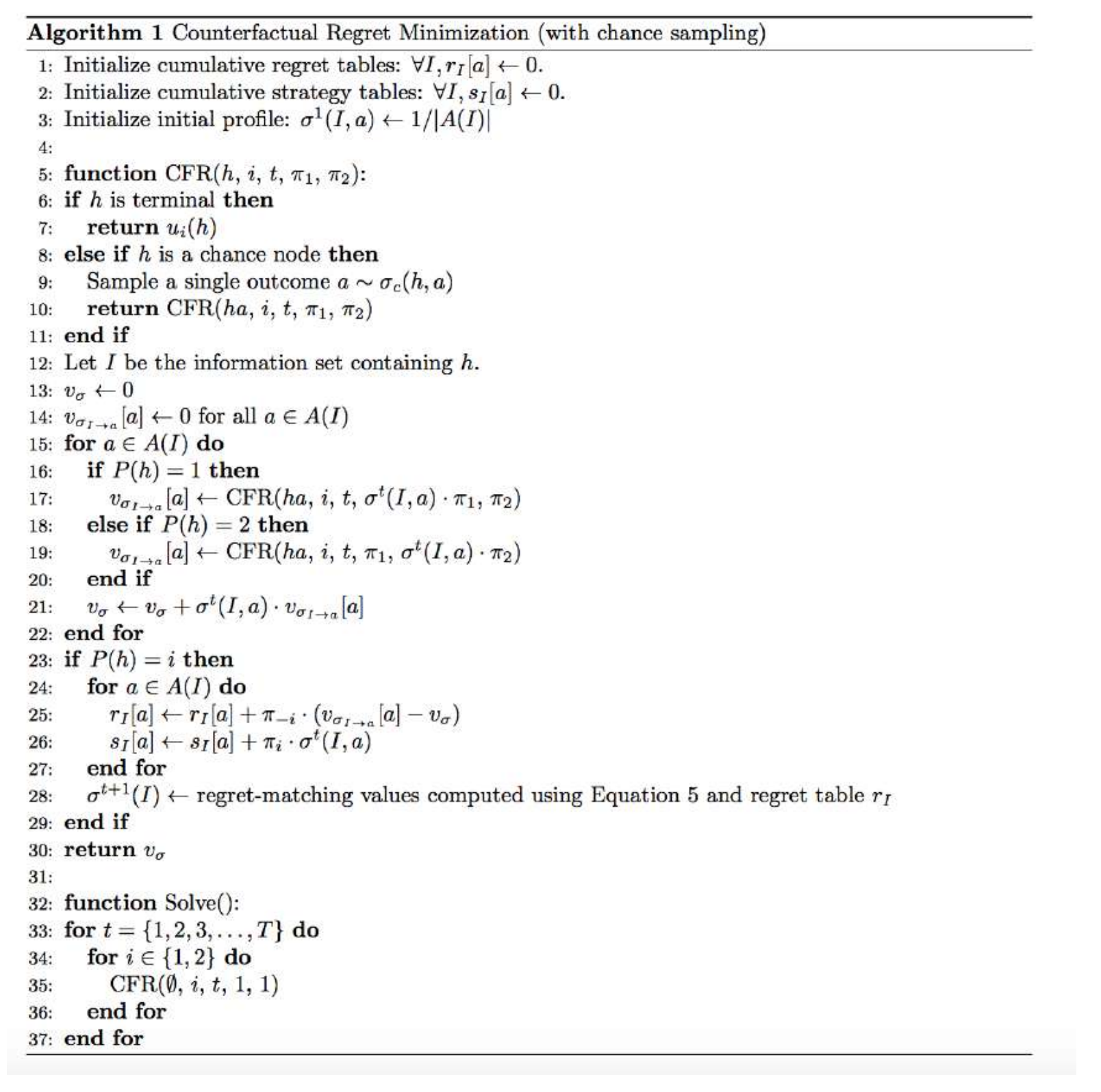
Code of the Vanilla version written in Java is available here.

Code including a best response function for the Chance Sampling algorithm is available here in Java.

Going through an Iteration

Here we show two full iterations of Chance Sampled CFR where we assume that the chance node has selected P1 Queen and P2 King as the random draw and then iterates over the entire tree from there.

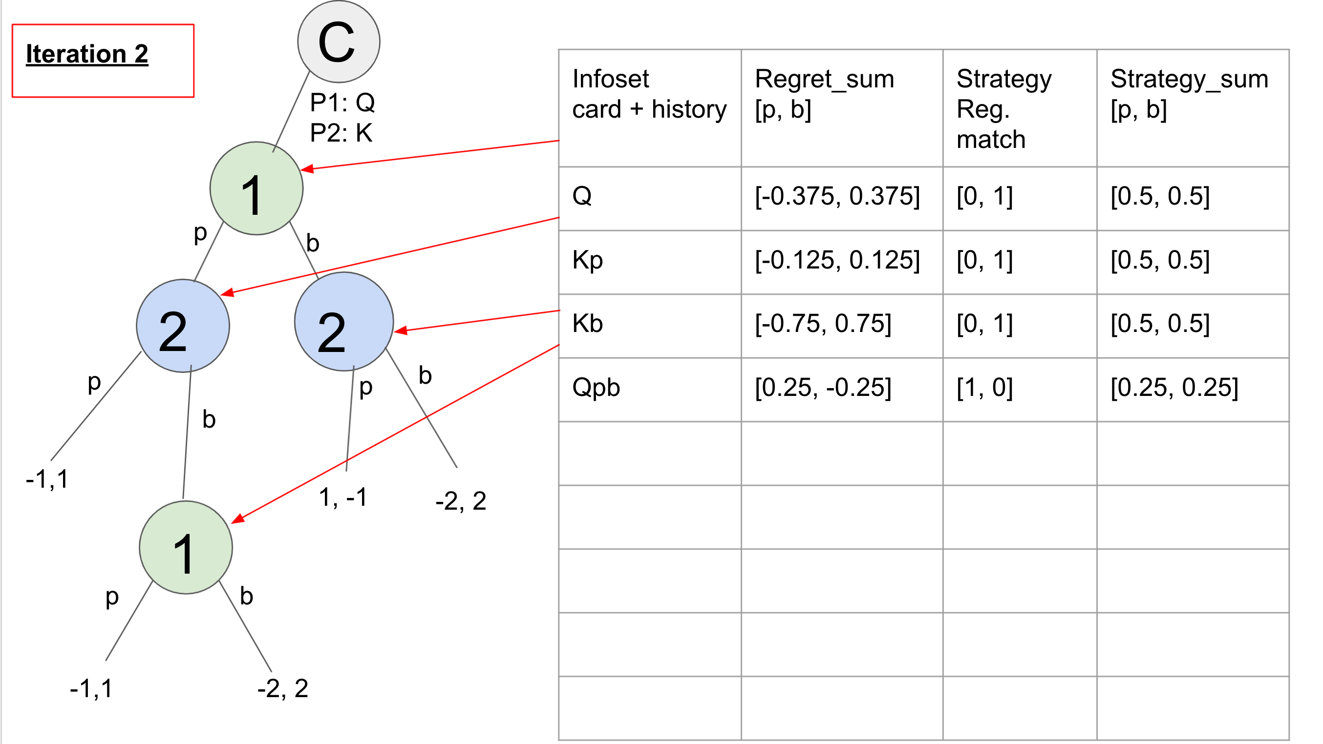
First we show the initialization of the algorithm which has four information sets (the card + the history of actions). At each information set the regret sum is stored where the first number represents the accumulated regret for passing and the second number represents the accumulated regret for betting. The strategy column is the behavioral strategy at that information set node, based on using regret matching with the accumulated regrets. Finally, the strategy sum is what we average at the end to find the Nash equilibrium strategy.

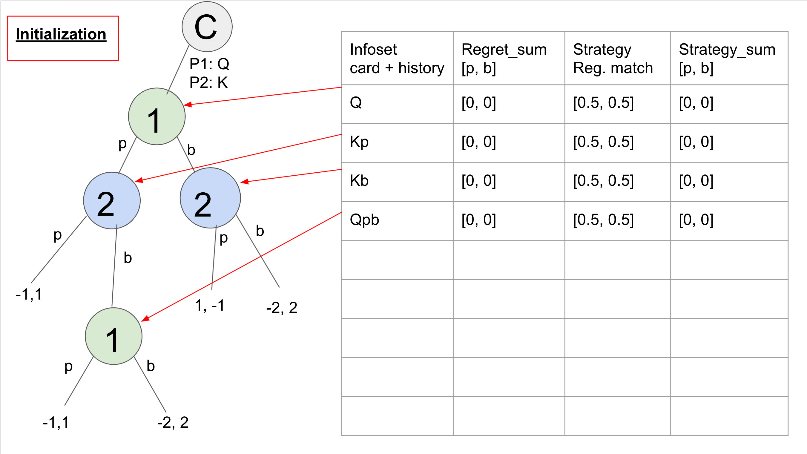
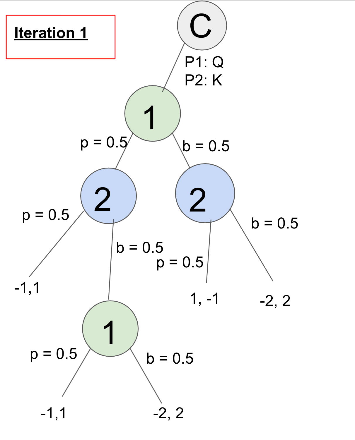
Here is the sequence of what the algorithm does in the first iteration:

Player 1 plays p = 0.5 at node Q.

Player 2 plays p = 0.5 at node Kp and gets utility of 1 for action p at node Kp.

Player 2 plays b = 0.5 at node Kp.

Player 1 plays p = 0.5 at node Qpb and gets utility of -1. Player 1 plays b = 0.5 at node Qpb and gets utility of -2. Node Qpb has overall utility of 0.5 * -1 + 0.5 * -2 = -1.5. Regret for playing p is -1 - (-1.5) = 0.5. Regret for playing b is -2 - (-1.5) = -0.5.

Regret_sum updates are regret * p(opponent playing to node) so here we have regret_sum[p] += 0.5 * 0.5 = 0.25 and regret_sum[b] += -0.5 * 0.5 = -0.25.

Node Qpb is valued at 1.5 for player 2 (opposite of what it was for player 1). Now from node Kp, player 2 had value 1 if playing p and value 1.5 if playing b, for a node_utility of 1.25. The regret for playing p is 1-1.25 = -0.25 and regret for playing b is 1.5-1.25 = 0.25.

Regret_sum updates are regret_sum[p] += -0.25 * 0.5 = -0.125 and regret_sum[b] += 0.25 * 0.5 = 0.125.

Node Kp is now valued at -1.25 for player 1 action p. Player 1 now takes action b = 0.5 from node Q. Then player 2 takes action p = 0.5 from node Kb and gets utility -1. Then player 2 takes action b = 0.5 from node Kb and gets utility 2. The node_util is 0.5. Regret for playing p is -1 - 0.5 = -1.5. Regret for playing b is 2 - 0.5 = 1.5.

Regret_sum updates are regret_sum[p] += -1.5 * 0.5= -0.75 and regret_sum[b] += 1.5 * 0.5 = 0.75.

Node Kb is now valued at -0.5 for player 1 action b. The node_util for node Q is 0.5 * -1.25 for action p and -0.5 * 0.5 for action b = -0.875. Regret for playing p is -1.25 - (-0.875) = -0.375 and regret for playing b is -0.5 - (-0.875) = 0.375. Regret_sum updates are regret_sum[p] += -0.375

Strategy_sum updates are probabilities of the node player not including the opponent playing to that action. So after this iteration each node was updated to [0.5, 0.5] except for the bottom node Qpb, which is [0.25, 0.25] since reaching that node comes after playing p = 0.5 in node Q, so both are 0.5 * 0.5.

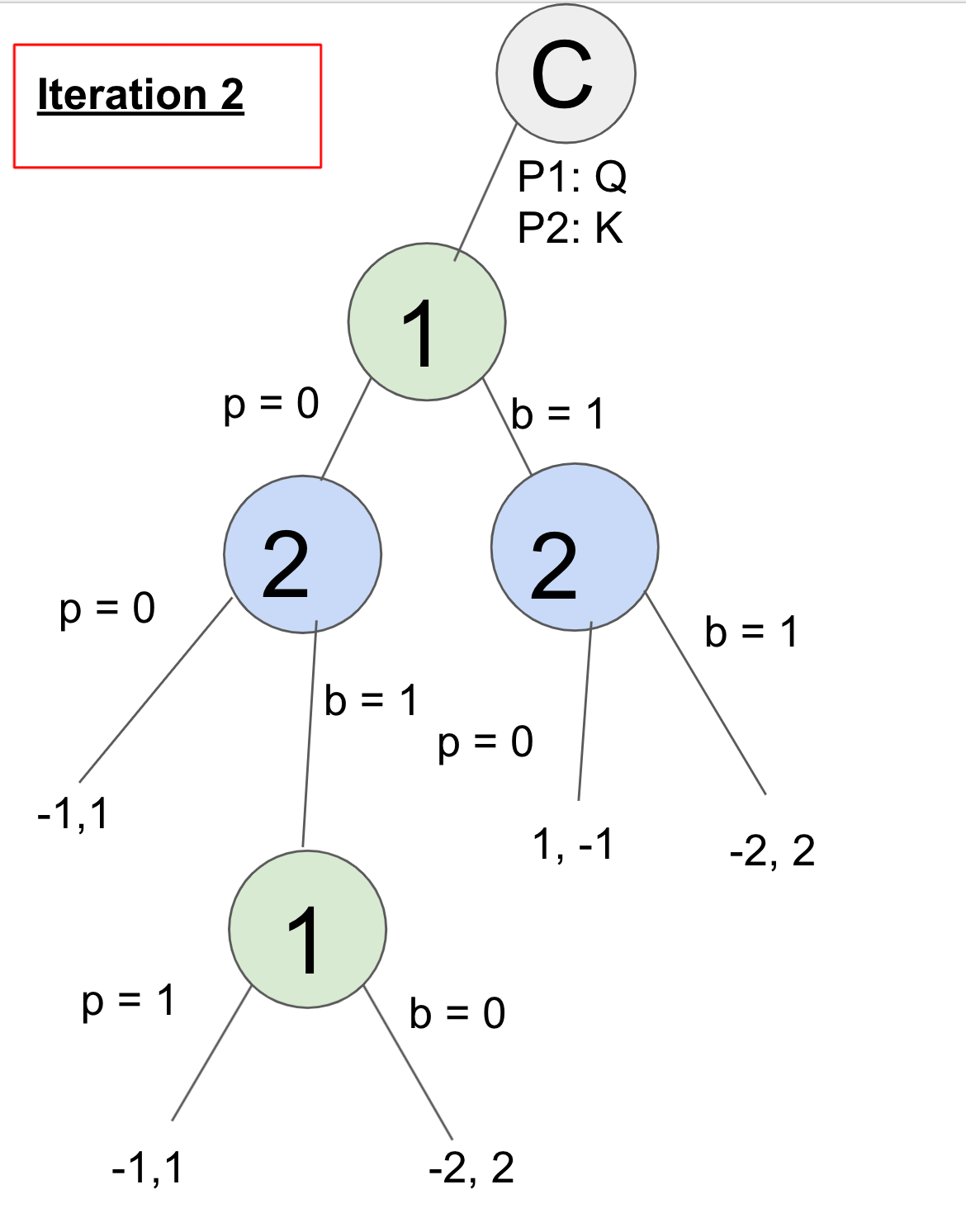
Player 1 plays p = 0 at node Q.

Player 2 plays p = 0 at node Kp and gets utility of 1.

Player 2 plays b = 0.5 at node Kp.

Player 1 plays p = 0.5 at node Qpb and gets utility of -1. Player 1 plays b = 0.5 at node Qpb and gets utility of -2. Node Qpb has overall utility of 0.5 * -1 + 0.5 * -2 = -1.5. Regret for playing p is -1 - (-1.5) = 0.5. Regret for playing b is -2 - (-1.5) = -0.5.

Regret_sum updates are regret * p(opponent playing to node) so here we have regret_sum[p] += 0.5 * 0.5 = 0.25 and regret_sum[b] += -0.5 * 0.5 = -0.25.

Node Qpb is valued at 1.5 for player 2 (opposite of what it was for player 1). Now from node Kp, player 2 had value 1 if playing p and value 1.5 if playing b, for a node_utility of 1.25. The regret for playing p is 1-1.25 = -0.25 and regret for playing b is 1.5-1.25 = 0.25.

Regret_sum updates are regret_sum[p] += -0.25 * 0.5 = -0.125 and regret_sum[b] += 0.25 * 0.5 = 0.125.

Node Kp is now valued at -1.25 for player 1 action p. Player 1 now takes action b = 0.5 from node Q. Then player 2 takes action p = 0.5 from node Kb and gets utility -1. Then player 2 takes action b = 0.5 from node Kb and gets utility 2. The node_util is 0.5. Regret for playing p is -1 - 0.5 = -1.5. Regret for playing b is 2 - 0.5 = 1.5.

Regret_sum updates are regret_sum[p] += -1.5 * 0.5= -0.75 and regret_sum[b] += 1.5 * 0.5 = 0.75.

Node Kb is now valued at -0.5 for player 1 action b. The node_util for node Q is 0.5 * -1.25 for action p and -0.5 * 0.5 for action b = -0.875. Regret for playing p is -1.25 - (-0.875) = -0.375 and regret for playing b is -0.5 - (-0.875) = 0.375. Regret_sum updates are regret_sum[p] += -0.375

Strategy_sum updates are probabilities of the node player not including the opponent playing to that action. So after this iteration each node was updated to [0.5, 0.5] except for the bottom node Qpb, which is [0.25, 0.25] since reaching that node comes after playing p = 0.5 in node Q, so both are 0.5 * 0.5.

Comparing Algorithms

We compared four CFR algorithms (Chance Sampling, External Sampling, Vanilla, and CFR+) in terms of exploitability vs. nodes touched (a measure of how long the algorithm has been running for) and then also look at two of those algorithms which are very similar, CFR and its recent update, CFR+, in terms of exploitability vs. time. Finally, we produce strategy charts that show a Nash equilibrium strategy for each player at all four stages of the game. CFR+ is explained more in the CFR Advances section, but in short resets regrets that have gone negative to 0 so they are more likely to have a chance to “rebound” in case they were actually good strategies that, for example, just got unlucky.

The simulations run for a set number of iterations and the regrets for all algorithms are updated after each iteration.

As the algorithms run, a best response function is called periodically, which iterates once through the game tree once for each player. The average of the best response values from each player is taken as the exploitability of the game at that point. All graphs show exploitability on the vertical axis on a log scale. CFR and CFR+ were run for 100,000 iterations and Chance and External Sampling were run for 10^9 iterations. Since the non-sampling algorithms require entire tree traversals for each iteration, they require far fewer iterations to reach the same number of nodes. The game value for all variants is -0.0566, as we have found in previous sections.

We examine nodes touched vs. exploitability for all four of our CFR algorithm types (Vanilla CFR vs. CFR+ vs. Chance Sampling vs. External Sampling) up to 4 * 10^9 nodes touched for each. Monte Carlo sampling methods require many more iterations than Vanilla CFR, while each iteration is relatively fast. Therefore, a nodes touched metric makes sense as a way of comparison.

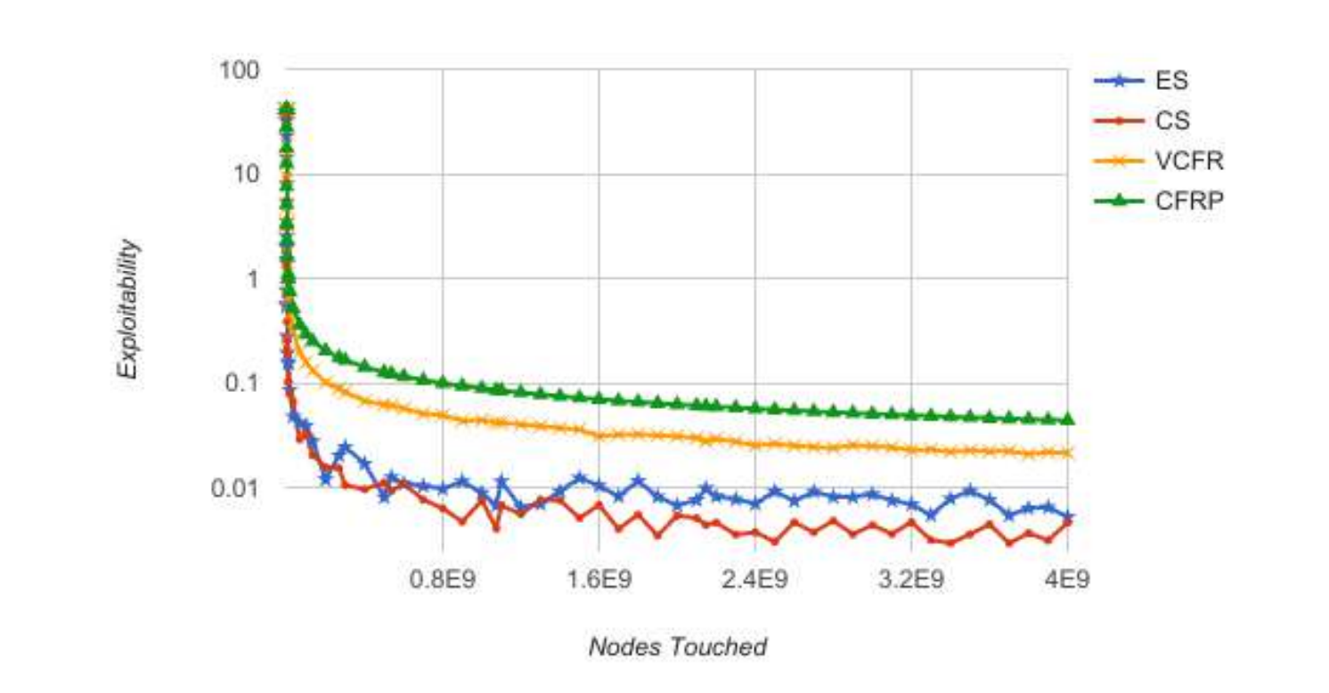
We can see that the sampled versions show a lower exploitability much faster than the Vanilla and CFR+ versions, although they are more erratic due to the sampling. While Chance Sampling is generally superior to External Sampling, they are quite close at the end of the experiment. Chance Sampling is the simplest algorithm, which may work in its favor since Kuhn Poker is also a very simple game. Vanilla CFR shows consistently lower exploitability than CFR+. Perhaps this is because CFR+ doesn’t allow regrets to become negative, it may then waste time on actions that would have gone negative.

We also experimented with time vs. exploitability. The algorithms and code for CFR+ and CFR are exactly the same except for how the regret is calculated and since this eliminates other sources of variability, we are able to reasonably compare CFR and CFR+ exploitability against time.

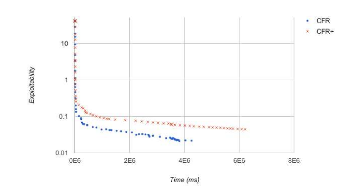
This graph shows that CFR+ takes significantly more time to complete its 100,000 iterations and yet is still at a higher exploitability. Since the only difference in the algorithms is that CFR+ does not allow regrets to become negative, this must be the cause of the additional calculation time needed.

Similarities with Reinforcement Learning

In reinforcement learning, agents learn what actions to take in an environment based on the rewards they’ve seen in the past. This is very similar to how regret updates work in CFR – we can think of the regrets as advantage functions, which is the value of a certain action compared to the value of a state, and in fact this terminology has been seen in recent papers like the Deep CFR paper. We can also compare this to having independent multiarm bandits at each decision point, learning from all of them simultaneously.