AIPT Section 2.1: Game Theory – Game Theory Foundation
Game Theory – Game Theory Foundation
Let’s look at some important game theory concepts before we get into actually solving for poker strategies.
Game Theory Optimal (GTO)
What does it mean to “solve” a poker game? In the 2-player setting, this means to find a Nash Equilibrium strategy (aka GTO strategy) for the game. By definition, if both players are playing this strategy, then neither would want to change to a different strategy since neither could do better with any other strategy (assuming that the opponent’s strategy stays fixed).
To break this down, if players A and B are both playing GTO, then both are doing as well as possible. If player A changes strategy, then player A is doing worse and player B is doing better. Player B could do even better by changing strategy to exploit player A’s new strategy, but then player A could take advantage of this change. If Player B stays put with GTO, then EV is not maximized, but there is no risk of being exploited. In this sense, GTO is an unexploitable strategy that gets a guaranteed minimum EV.
With more than 2 players, Nash equilibria are still guaranteed to exist, but algorithms that work to solve 2 player games are not guaranteed to converge to the equilibrium strategy, though the strategies still tend to be strong. Even if you did know a Nash equilibrium strategy for your own position in a multiplayer game, other players could either (a) play strategies that weaken your expected value or (b) play their own Nash equilibrium strategies but the resulting combination of strategies is not guaranteed to be a Nash equilibrium.
In practice, even in the 2-player setting, we have to approximate GTO strategies in full-sized poker games. We will go more into the details of what it means to solve a game in section 3.1 “What is Solving”?
Intuition for equilibrium in poker can be explained using a simple all-in game where one player must either fold or bet all his chips and the second player must either call or fold if the first player bets all the chips. We’ll refer to these two players as the “all-in player” and the “calling player”. We assume each player starts with 10 big blinds and P1 puts in a small blind of 0.5 units and P2 puts in a big blind of 1 unit. There are three possible outcomes:
| Scenarios | Player 1 (SB) | Player 2 (BB) | Result |
|---|---|---|---|
| Case 1 | Fold | – | P2 wins 0.5 BB |
| Case 2 | All-in | Fold | P1 wins 1 BB |
| Case 3 | All-in | Call | Winner of showdown wins 10 BB (pot size 20 BB) |
In this situation, the calling player might begin the game with a default strategy of calling a low percentage of hands. An alert all-in player might exploit this by going all-in with a large range of hands.
After seeing the first player go all-in very frequently, the calling player might increase the calling range.
Once the all-in player observes this, it could lead him to reduce his all-in percentage. Once the all-in range of hands and the calling range stabilize such that neither player can unilaterally change his strategy to increase his profit, then the equilibrium strategies have been reached.
A strategy in game theory is the set of actions one will take at every decision point. In the all-in game, there is only one decision for each player, so the entire strategy is the number of hands to go all-in with for Player 1 and the number of hands to call with for Player 2. A real strategy in poker would say what to do with every possible hand in every situation. For example, it might say that when you have 98 suited on the button and it’s folded to you, you should raise 2.5x the pot 90% of the time and go allin 10% of the time.
We can use the ICMIZER program to compute the game theory optimal strategies in a 1v1 setting where both players start the hand with 10 big blinds. In this case, the small blind all-in player goes all-in 58% of the time and the big blind calling player calls 37% of the time.
If either player changed those percentages, then their EV would go down! If the calling player called more hands (looser), those hands wouldn’t be profitable. If the calling player called fewer hands (tighter), then he would be folding too much. If the all-in player went looser, those extra hands wouldn’t be profitable, and if he went tighter, then he would be folding too much.
Why, intuitively, is the all-in player’s range so much wider than the calling player’s? David Sklansky coined the term “gap concept”, which states that a player needs a better hand to call with than to go all-in with – that difference is the gap. The main reasons for this are (a) the all-in player gets the initiative whereby he can force a fold, but the calling player can only call, (b) the all-in player is signaling the strength of his hand, and (c) when facing an all-in bet the pot odds are not especially appealing.
Exploitation
What if the big blind calling player doesn’t feel comfortable calling with weaker hands like K2s and Q9o and maximized his calling range tighter than the equilibrium range of 37%? The game theoretic solution strategy for the other player would not fully take advantage of this opportunity. The best response strategy is the one that maximally exploits the opponent by always performing the highest expected value play against their fixed strategy. In general, an exploitative strategy is one that exploits an opponent’s non-equilibrium play. In the above example, an exploitative play could be raising with all hands after seeing the opponent calling with a low percentage of hands. However, this strategy can itself be exploited. When both players are playing a Nash equililbrium then they are playing best response strategies against each other.
Normal Form
Normal Form is writing the strategies and game payouts in matrix form. The Player 1 strategies are in the rows and Player 2 strategies are in the columns. The payouts are written in terms of P1, P2.
Zero-Sum All-in Poker Game
We can model the all-in game in normal form as below. Assume that each player looks at his/her hand and settles on an action, then the below chart is the result of those actions with the first number being Player 1’s payout and the second being Player 2’s. In general, normal form matrices show utilities for each player in a game, which is what the situation is valued for each player, and in poker settings, these are the payouts from the hand.
Note that e.g. the call player cannot call when the all-in player folds, but we assume the actions are pre-selected and the payouts still remain the same.
In a one on one poker game, the sum of the payouts in each box are 0 since whatever one player wins, the other loses, which is called a zero-sum game (not including the house commission, aka rake).
| All-in Player/Call Player | Call | Fold |
|---|---|---|
| All-in | EV of all-in, -EV of all-in | 1, -1 |
| Fold | -0.5, 0.5 | -0.5, 0.5 |
If Player 1 has JT offsuit and Player 2 has AK offsuit, the numbers are as below. The all-in call scenario has -2.5 for Player 1 and 2.5 for Player 2 because the hand odds are about 37.5% for Player 1 and 62.5% for Player 2, meaning that Player 1’s equity in a \$20 pot is about \$7.50 and Player 2’s equity is about $12.50, so the net expected profit is -\$2.50 and \$2.50, respectively.
| All-in Player/Call Player | Call | Fold |
|---|---|---|
| All-in | -2.5, 2.5 | 1, -1 |
| Fold | -0.5, 0.5 | -0.5, 0.5 |
Because in poker the hands are hidden, there would be no way to actually know the all-in/call EV in advance, but we show this to understand how the normal form looks.
Simple 2-Action Game
| P1/P2 | Action 1 | Action 2 |
|---|---|---|
| Action 1 | 5, 3 | 4, 0 |
| Action 2 | 3, 2 | 1, -1 |
In the Player 1 Action 1 and Player 2 Action 1 slot, we have (5, 3), which represents P1 = 5 and P2 = 3. I.e., if these actions are taken, Player 1 wins 5 units and Player 2 wins 3 units.
Dominated Strategies
A dominated strategy is one that is strictly worse than an alternative strategy. Let’s find the equilibrium strategies for this game by using iterated elimination of dominated strategies.
If Player 2 plays Action 1, then Player 1 gets a payout of 5 with Action 1 or 3 with Action 2. Therefore Player 1 prefers Action 1 in this case.
If Player 2 plays Action 2, then Player 1 gets a payout of 4 with Action 1 or 1 with Action 2. Therefore Player 1 prefers Action 1 again in this case.
This means that whatever Player 2 does, Player 1 prefers Action 1 and therefore can eliminate Action 2 entirely since it would never make sense to play Action 2. We can say Action 1 dominates Action 2 or Action 2 is dominated by Action 1.
We can repeat the same process for Player 2. When Player 1 plays Action 1, Player 2 prefers Action 1 (3>0). When Player 1 plays Action 2, Player 2 prefers Action 1 (2>-1). Even though we already established that Player 1 will never play Action 2, Player 2 doesn’t know that so needs to evaluate that scenario.
We see that Player 2 will also always play Action 1 and has eliminated Action 2.
Therefore we have an equilibrium at (5,3) and no player would want to deviate or else they would have a lower payout!
3-Action Game
In the Player 1 Action 1 and Player 2 Action 1 slot, we have (10, 2), which represents P1 = 10 and P2 = 2. I.e. if these actions are taken, Player 1 wins 10 units and Player 2 wins 2 units.
| P1/P2 | Action 1 | Action 2 | Action 3 |
|---|---|---|---|
| Action 1 | 10, 2 | 8, 1 | 3, -1 |
| Action 2 | 5, 8 | 4, 0 | -1, 1 |
| Action 3 | 7, 3 | 5, -1 | 0, 3 |
Given this table, how can we determine the best actions for each player? Again, P1 is represented by the rows and P2 by the columns.
We can see that Player 1’s strategy of Action 1 dominates Actions 2 and 3 because all of the values are strictly higher for Action 1. Regardless of Player 2’s action, Player 1’s Action 1 always has better results than Action 2 or 3.
When P2 chooses Action 1, P1 earns 10 with Action 1, 5 with Action 2, and 7 with Action 3 When P2 chooses Action 2, P1 earns 8 with Action 1, 4 with Action 2, and 5 with Action 3 When P2 chooses Action 3, P1 earns 7 with Action 1, 5 with Action 2, and 0 with Action 3
We also see that Action 1 dominates Action 2 for Player 2. Action 1 gets payouts of 2 or 8 or 3 depending on Player 1’s action, while Action 2 gets payouts of 1 or 0 or -1, so Action 1 is always superior.
Action 1 weakly dominates Action 3 for Player 2. This means that Action 1 is greater than or equal to playing Action 3. In the case that Player 1 plays Action 3, Player 2’s Action 1 and Action 3 both result in a payout of 3 units.
We can eliminate strictly dominated strategies and then arrive at the reduced Normal Form game. Recall that Player 1 would never play Actions 2 or 3 because Action 1 is always better. Similarly, Player 2 would never play Action 2 because Action 1 is always better.
| P1/P2 | Action 1 | Action 3 |
|---|---|---|
| Action 1 | 10, 2 | 3, -1 |
In this case, Player 2 prefers to play Action 1 since 2 > -1, so we have a Nash Equilibrium with both players playing Action 1 100% of the time (also known as a pure strategy) and the payouts will be 10 to Player 1 and 2 to Player 2. The issue with Player 2’s Action 1 having a tie with Action 3 when Player 1 played Action 3 was resolved because we now know that Player 1 will never actually play that action and when Player 1 plays Action 1, Player 2 will always prefer Action 1 to Action 3.
| P1/P2 | Action 1 |
|---|---|
| Action 1 | 10, 2 |
To summarize, Player 1 always plays Action 1 because it dominates Actions 2 and 3. When Player 1 is always playing Action 1, it only makes sense for Player 2 to also play Action 1 since it gives a payoff of 2 compared to payoffs of 1 and -1 with Actions 2 and 3, respectively.
Tennis vs. Power Rangers
In this game, we have two people who are going to watch something together. P1 has a preference to watch tennis and P2 prefers Power Rangers. If they don’t agree, then they won’t watch anything and will have payouts of 0. If they do agree, then the person who gets to watch their preferred show has a higher reward than the other, but both are positive.
| P1/P2 | Tennis | Power Rangers |
|---|---|---|
| Tennis | 3, 2 | 0, 0 |
| Power Rangers | 0, 0 | 2, 3 |
In this case, neither player can eliminate a strategy. For Player 1, if Player 2 chooses Tennis then he also prefers Tennis, but if Player 2 chooses Power Rangers, then he prefers Power Rangers as well (both of these are Nash Equilbrium). This is intuitive (assuming that the payouts are valid, i.e., that the people really like TV) because there is 0 value in watching nothing but at least some value if both agree to watch one thing. This also shows the Nash equilibrium principle of not being able to benefit from unilaterally changing strategies – if both are watching tennis and P2 changes to Power Rangers, that change would reduce value from 2 to 0!
So what is the optimal strategy here? If each player simply picked their preference, then they’d always watch nothing and get 0! If they both always picked their non-preference, then the same thing would happen! If they pre-agreed to either Tennis or Power Rangers, then utilties would increase, but this would never be “fair” to either person.
We can calculate the optimal strategies like this:
Let’s define:
\[\text{P(P1 Tennis)} = p\] \[\text{P(P1 Power Rangers)} = 1 - p\]These represent the probability that Player 1 would select each of these.
If Player 2 chooses Tennis, Player 2 earns \(p*(2) + (1-p)*(0) = 2p\). The EV is calculated as probabilities of Player 1 multiplied by payouts of Player 2 playing Tennis.
If Player 2 chooses Power Rangers, Player 2 earns \(p*(0) + (1-p)*(3) = 3 - 3p\)
We are trying to find a strategy that involves mixing between both options, a mixed strategy. A fundamental rule is that if you are going to play multiple strategies, then the utility value of each must be the same, because otherwise you would just pick one and stick with that.
Therefore we can set these values equal to each other, so
\[2p = 3 - 3p\] \[5p = 3\] \[p = 3/5\]Therefore Player 1’s strategy is to choose Tennis \(p = 3/5\) and Power Rangers \(1 - p = 2/5\). This is a mixed strategy equilibrium because there is a probability distribution over which strategy to play.
This result comes about because these are the probabilities for P1 that induce P2 to be indifferent between Tennis and Power Rangers.
By symmetry, P2’s strategy is to choose Tennis \(2/5\) and Power Rangers \(3/5\).
This means that each player is choosing his/her chosen program \(3/5\) of the time, while choosing the other option \(2/5\) of the time. Let’s see how the final outcomes look.
Tennis, Tennis occurs \(3/5 * 2/5 = 6/25\)
Power Rangers, Power Rangers occurs \(2/5 * 3/5 = 6/25\)
Tennis, Power Rangers occurs \(3/5 * 3/5 = 9/25\)
Power Rangers, Tennis occurs \(2/5 * 2/5 = 4/25\)
These probabilities are shown below (this is not a normal form matrix because we are showing probabilities and not payouts):
| P1/P2 | Tennis | Power Rangers |
|---|---|---|
| Tennis | 6/25 | 9/25 |
| Power Rangers | 4/25 | 6/25 |
The average payouts to each player are \(6/25 * (3) + 6/25 * (2) = 30/25 = 1.2\). This would have been higher if they had avoided the 0,0 payouts! Unfortunately \(9/25 + 4/25 = 13/25\) of the time, the payouts were 0 to each player. Coordinating to watch something rather than so often watching nothing would be a much better solution!
What if Player 1 decided to be sneaky and change his strategy to choosing Tennis always instead of \(3/5\) tennis and \(2/5\) Power Rangers? Remember that there can be no benefit to deviating from a Nash Equilibrium strategy by definition. If he tries this, then we have the following likelihoods since P1 is never choosing Power Rangers and so the probabilities are determined strictly by P2’s strategy of \(2/5\) tennis and \(3/5\) Power Rangers:
| P1/P2 | Tennis | Power Rangers |
|---|---|---|
| Tennis | 2/5 | 3/5 |
| Power Rangers | 0 | 0 |
The Tennis and Power Rangers \(3/5\) has no payoffs and the Tennis Tennis has a payoff of of \(2/5 * 3 = 6/5 = 1.2\) for P1. This is the same as the payout he was already getting. Note that deviating from the equilibrium can maintain the same payoff, but cannot improve the payoffs. In the zero-sum case, the opponent also can only do better or equal when a player deviates, but in this case Player 2 actually has a lower payoff of \(2/5 * 2 = 0.8\) instead of \(1.2\).
However, P2 might catch on to this and then get revenge by pulling the same trick and changing strategy to always selecting Power Rangers, resulting in the following probabilities:
| P1/P2 | Tennis | Power Rangers |
|---|---|---|
| Tennis | 0 | 1 |
| Power Rangers | 0 | 0 |
Now the probability is fully on P1 picking Tennis and P2 picking Power Rangers, and nobody gets anything!
Rock Paper Scissors
Finally, we can also think about this concept in Rock-Paper-Scissors. Let’s define a win as +1, a tie as 0, and a loss as -1. The game matrix for the game is shown below in Normal Form:
| P1/P2 | Rock | Paper | Scissors |
|---|---|---|---|
| Rock | 0, 0 | -1, 1 | 1, -1 |
| Paper | 1, -1 | 0, 0 | -1, 1 |
| Scissors | -1, 1 | 1, -1 | 0, 0 |
As usual, Player 1 is the row player and Player 2 is the column player. The payouts are written in terms of P1, P2. So for example P1 Paper and P2 Rock corresponds to a reward of +1 for P1 and -1 for P2 since Paper beats Rock.
The equilibrium strategy is to play each action with \(1/3\) probability. We can see this intuitively because if any player played anything other than this distribution, then you could crush them by always playing the strategy that beats the strategy that they most favor. For example if someone played rock 50%, paper 25%, and scissors 25%, they are overplaying rock, so you could always play paper and then would win 50% of the time, tie 25% of the time, and lose 25% of the time for an average gain of \(1*0.5 + 0*0.25 + (-1)*0.25 = 0.25\) each game.
| P1/P2 | Rock 50% | Paper 25% | Scissors 25% |
|---|---|---|---|
| Rock 0% | 0 | 0 | 0 |
| Paper 100% | 0.5*1 = 0.5 | 0.25*0 = 0 | 0.25*(-1) = -0.25 |
| Scissors 0% | 0 | 0 | 0 |
We can also work it out mathematically. Let P1 play Rock \(r%\), Paper \(p%\), and Scissors \(s%\). The utility of P2 playing Rock is then \(0*(r) + -1 * (p) + 1 * (s)\). The utility of P2 playing Paper is \(1 * (r) + 0 * (p) + -1 * (s)\). The utility of P2 playing Scissors is \(-1 * (r) + 1 * (p) + 0 * (s)\).
We can figure out the best strategy with this system of equations (the second equation below is because all probabilities must add up to 1):
\[\begin{cases} -p + s = r - s = -r + p \\ r + p + s = 1 \end{cases}\] \[-p + s = r - s \implies 2s = p + r\] \[r - s = - r + p \implies 2r = s + p\] \[-p + s = -r + p \implies s + r = 2p\] \[r + s + p = 1 \implies r + s = 1 - p\]Setting the last two equations equal, we have:
\[1 - p = 2p\] \[1 = 3p\] \[p = 1/3\]Rewriting the final equation:
\[r + s + p = 1\] \[s + p = 1 - r\]Using the above combined with the 2nd equation:
\[1 - r = 2r\] \[1 = 3r\] \[1/3 = r\]Writing the probabability sums to 1 equation with the results for \(p\) and \(r\):
\[1/3 + 1/3 + s = 1 s = 1/3\]The equilibrium strategy is therefore to play each action with 1/3 probability.
If your opponent plays the equilibrium strategy of Rock 1/3, Paper 1/3, Scissors 1/3, then he will have the following EV. EV = \(1*(1/3) + 0*(1/3) + (-1)*(1/3) = 0\). Note that in Rock Paper Scissors, if you play equilibrium then you can never show a profit because you will always breakeven, regardless of what your opponent does. In poker, this is not the case.
Regret
When I think of regret related to poker, the first thing that comes to mind is often “Wow you should’ve played way more hands in 2010 when poker was so easy”. Often in poker we regret big folds or bluffs or calls that didn’t work out well (even though poker players in general are good at not being very results oriented).
Here we will look at a less sad version, the mathematical concept of regret. Regret is a measure of how well you could have done compared to some alternative. Phrased differently, what you would have done in some situation instead.
\(\text{Regret} = \text{u(Alternative Strategy)} - \text{u(Current Strategy)}\) where \(u\) represents utility
If your current strategy for breakfast is cooking eggs at home, then maybe \(\text{u(Current Home Egg Strategy)} = 5\). If you have an alternative of eating breakfast at a fancy buffet, then maybe \(\text{u(Alternative Buffet Strategy)} = 9\), so the regret for not eating at the buffet is \(9 - 5 = 4\). If your alternative is getting a quick meal from McDonald’s, then you might value \(\text{u(Alternative McDonald's Strategy)} = 2\), so regret for not eating at McDonald’s is \(2 - 5 = -3\). We prefer alternative actions with high regret.
We can give another example from Rock Paper Scissors:
We play rock and opponent plays paper \(\implies \text{u(rock,paper)} = -1\)
\[\text{Regret(scissors)} = \text{u(scissors,paper)} - \text{u(rock,paper)} = 1-(-1) = 2\] \[\text{Regret(paper)} = \text{u(paper,paper)} - \text{u(rock,paper)} = 0-(-1) = 1\] \[\text{Regret(rock)} = \text{u(rock,paper)} - \text{u(rock,paper)} = -1-(-1) = 0\]We play scissors and opponent plays paper \(\implies \text{u(scissors,paper)} = 1\)
\[\text{Regret(scissors)} = \text{u(scissors,paper)} - \text{u(scissors,paper)} = 1-1 = 0\] \[\text{Regret(paper)} = \text{u(paper,paper)} - \text{u(scissors,paper)} = 0-1 = -1\] \[\text{Regret(rock)} = \text{u(rock,paper)} - \text{u(scissors,paper)} = -1-1 = -2\]We play paper and opponent plays paper \(\implies \text{u(paper,paper)} = 0\)
\[\text{Regret(scissors)} = \text{u(scissors,paper)} - \text{u(paper,paper)} = 1-0 = 1\] \[\text{Regret(paper)} = \text{u(paper,paper)} - \text{u(paper,paper)} = 0-0 = 0\] \[\text{Regret(rock)} = \text{u(rock,paper)} - \text{u(paper,paper)} = -1-0 = -1\]Again, we prefer alternative actions with high regret.
To generalize for the Rock Paper Scissors case:
- The action played always gets a regret of 0 since the “alternative” is really just that same action
- When we play a tying action, the alternative losing action gets a regret of -1 and the alternative winning action gets a regret of +1
- When we play a winning action, the alternative tying action gets a regret of -1 and the alternative losing action gets a regret of -2
- When we play a losing action, the alternative winning action gets a regret of +2 and the alternative tying action gets a regret of +1
Bandits
A common way to analyze regret is the multi-armed bandit problem. The setup is a player sitting in front of a multi-armed “bandit” with some number of arms. (Think of this as sitting in front of a bunch of slot machines.) Each time the player pulls an arm, they get some reward, which could be positive or negative. Bandits are a set of problems with repeated decisions and a fixed number of actions possible. This is related to reinforcement learning because the agent player updates its strategy based on what it learns from the feedback from the environment.
Multi-armed bandit problems are a common representation of regret and an algorithm is called “no-regret” if its average overall regret grows sublinearly in time. In the adversarial setting, the opponent chooses the reward. This is the equivalent setting that we see in poker games, since the opponent’s actions influence our utility in the game.
In the full information setting, the player can see the entire reward vector for each machine chosen and in the partial setting, sees only the reward that the machine has chosen for that particular play. Here we will focus on the partial setting.
A basic setting initializes each of 10 arms with \(q_*(\text{arm}) = \mathcal{N}(0, 1)\), so each is initialized with a center point found from the Gaussian distribution. Each pull of an arm then gets a reward of \(R = \mathcal{N}(q_*(\text{arm}), 1)\).
To clarify, this means each arm is initialized with a value centered around 0 but with some variance, so each will be a bit different. Then from that point, the actual pull of an arm is centered around that new point with some variance as seen in this figure with a 10-armed bandit from Intro to Reinforcement Learning by Sutton and Barto:
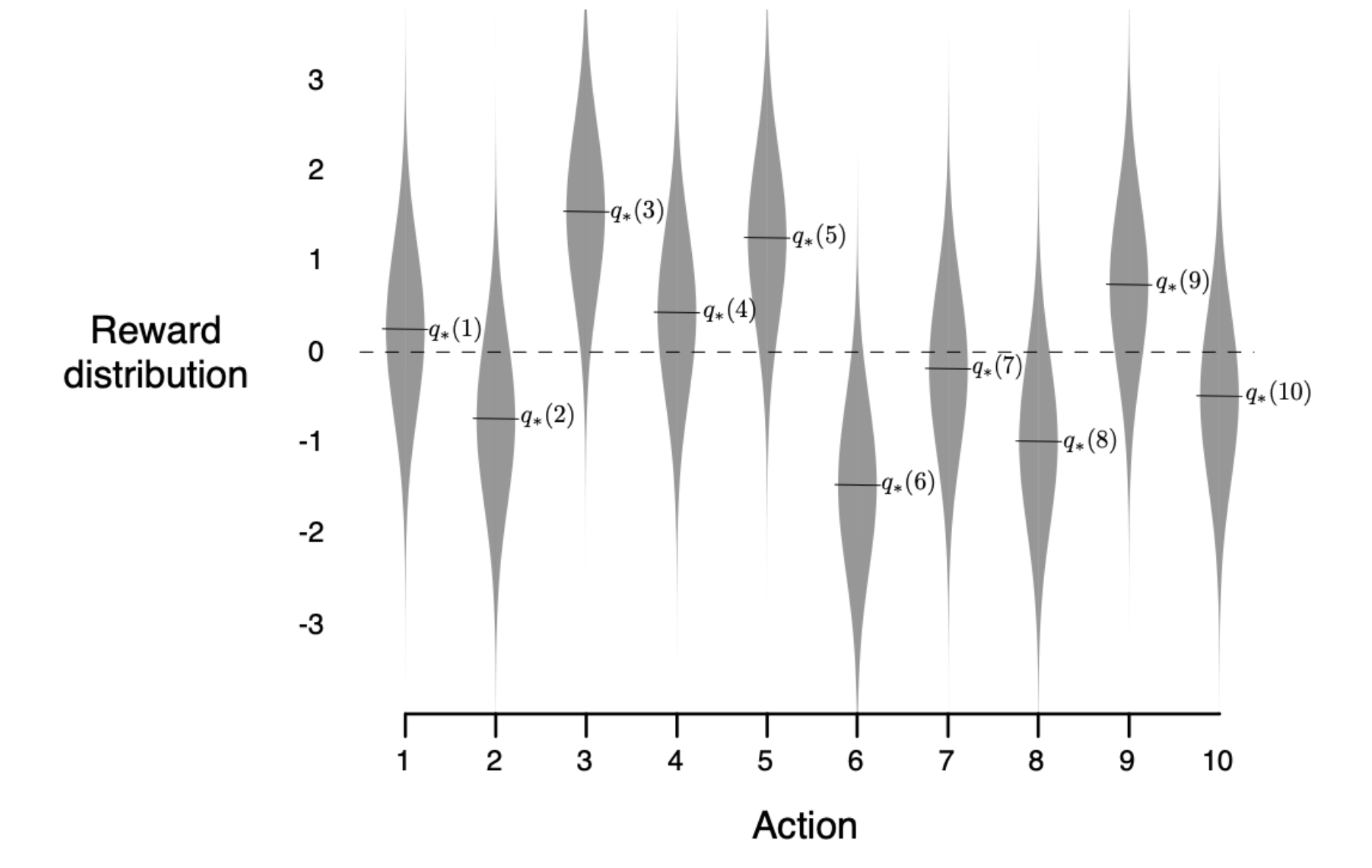
In simple terms, each machine has some set value that isn’t completely fixed at that value, but rather varies slightly around it, so a machine with a value of 3 might range from 2.5 to 3.5.
Imagine that the goal is to play this game 2000 times with the intention to achieve the highest rewards. We can only learn about the rewards by pulling the arms – we don’t have any information about the distribution behind the scenes. We maintain an average reward per pull for each arm as a guide for which arm to pull in the future.
Greedy The most basic algorithm to score well is to pull each arm once and then forever pull the arm that performed the best in the sampling stage. This could be modified by pulling each arm \(n\) times and then pulling the best arm, while allowing “best arm” to be updated if the average reward for the current best arm becomes worse than another arm. If multiple actions have the same value, then select either the lowest index or one of the ties at random.
Epsilon Greedy \(\epsilon\)-Greedy works similarly to Greedy, but instead of always picking the best arm, we use an \(\epsilon\) value that defines how often we should randomly pick a different arm. We keep track of which arm is the current best arm before each pull according to the average reward per pull, then play that arm \(1-\epsilon\) of the time and play a random arm \(\epsilon\) of the time. For example if \(\epsilon\) was 0.1, then we’d pick the currently known best arm 90% of the time and a random arm 10% of the time.
The idea of usually picking the best arm and sometimes switching to a random one is the concept of exploration vs. exploitation. Think of this in the context of picking a travel destination or picking a restaurant. You are likely to get a very high “reward” by continuing to go to a favorite vacation spot or restaurant, but it’s also useful to explore other options that you could end up preferring. (Note to self: Think about not eating the same exact meals every day.)
This idea is also seen in online advertising, where an advertiser might create a few ads for the same product, then show a random one for each user on the site. They could then monitor which ones get the most clicks and therefore which ones tend to work better than the others. Should they greedily “exploit” by using the best-ranked ad or continue accumulating data or use some kind of epsilon Greedy method that now mostly uses the best ad but also sometimes shows other ones to accumulate more data?
Bandit Regret The goal of the agent playing this game is to get the best reward. This is done by pulling the best arm repeatedly, but this is of course not known to the agent in advance. We can define a very sensible definition of average regret as
\[\text{Regret}_t = \frac{1}{t} \sum_{\tau=1}^t (V^* - Q(a_\tau))\]where \(V^*\) is the fixed reward from the best action, \(Q(a_\tau)\) is the reward from selecting arm \(a\) at timestep \(\tau\), and \(t\) is the total number of timesteps.
So at each timestep, we are computing the difference between if we had picked the best possible action (for the sake of the calculation we assume that we are able to know this) compared to the actual action that we pulled and taking the average.
In other words, this is the average of how much worse we have done than the best possible action over the number of timesteps.
So if the best action would give a value of 5 and our rewards on our first 3 pulls were {3, 5, 1}, our regrets would be {5-3, 5-5, 5-1} = {2, 0, 4}, for an average of \((2+0+4)/3 = 2\). So the equivalent to trying to maximize rewards is trying to minimize regret.
Note that above we said that the idea was to maximize regret and that we’d play actions in proportion to the regrets with regret matching. Now we’re trying to minimize regret. This is confusing and regret can be interpreted in both ways depending on the situation.
For values of \(\epsilon = 0\) (greedy), \(\epsilon = 0.01\), \(\epsilon = 0.1\), and \(\epsilon = 0.5\) and using the setup described above, we did a simulation that averaged 2,000 runs of 1,000 timesteps each.
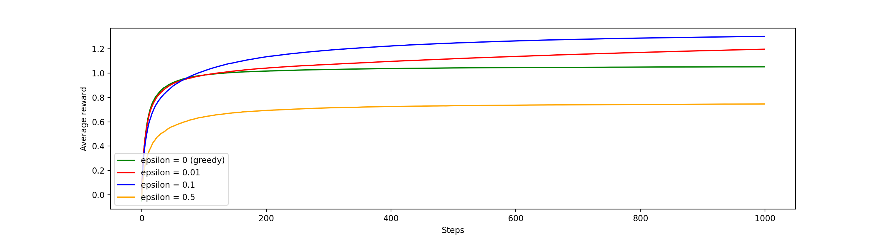 Average reward plot
For the average reward plot, we see that the optimal \(\epsilon\) amongst those used is 0.1, next best is 0.01, then 0, and then 0.5. This shows that some exploration is valuable, but too much (0.5) or too little (0) is not optimal.
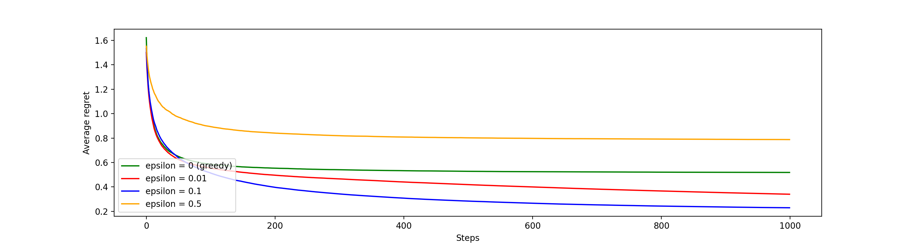 Average regret plot
The average regret plot is the inverse of the reward plot because it is the best possible reward minus the actual rewards received and so the goal is to minimize the regret.
Upper Confidence Bound (UCB) There are many algorithms for choosing bandit arms. The last one we’ll touch on is called Upper Confidence Bound (UCB). This bound represents that even though we have some data about the value of an arm, there is some uncertainty around it so we can take the upper bound of this uncertainty to determine which arm to pull next.
\[A_t = \arg\max_{a}(Q_t(a) + c*\sqrt{\frac{log{t}{N_t(a)}})\]The output of the formula is to choose the optimal action. The \(Q_{t(a)}\) represents the exploitation – it is the average value so far of the pulls from playing action \(a\) at time \(t\). The rest of the equation represents the exploration and \(c\) is the exploration constant. The \(t\) term in the numerator represents the number of pulls completed so far in total (not just for a particular action) and the denominator term represents the number of pulls for action \(a\). This means that for actions that have been pulled less, the term will be higher (we are more uncertain about the true value of that action).
The Upper Confidence Bound formula effectively selects the action that has the highest estimated value (exploitation) plus the upper confidence bound exploration term. We can think of this sort of as a “maximum expectation” or “optimism in the face of uncertainty” term and therefore would choose to pull the next arm that has the highest upper confidence bound value, and the equation for that arm would be updated after each pull with the new \(Q_{t(a)}\) estimate and new values of \(t\) and \(N_{t(a)}\).
Regret Matching
The concept of regret matching was developed in 2000 by Hart and Mas-Collel. Regret matching means playing a future strategy in proportion to the accumulated regrets from past actions. As we play, we keep track of the accumulated regrets for each action and then play in proportion to those values. For example, if the total regret values for Rock are 5, Paper 10, Scissors 5, then we have total regrets of 20 and we would play Rock 5/20 = 1/4, Paper 10/20 = 1/2, and Scissors 5/20 = 1/4.
It makes sense intuitively to prefer actions with higher regrets because they provide higher utility, as shown in the prior section. So why not just play the highest regret action always or with some epsilon? Because playing in proportion to the regrets allows us to keep testing all of the actions, while still more often playing the actions that have the higher chance of being best. It could be that at the beginning, the opponent happened to play Scissors 60% of the time even though their strategy in the long run is to play it much less. We wouldn’t want to exclusively play Rock in this case, we’d want to keep our strategy more robust. It also means that we aren’t as predictable.
The regret matching algorithm works like this:
- Initialize regret for each action to 0
- Set the strategy as: \(\text{strategy} _{action}_{i} = \begin{cases} \frac{R_{i}^{+}}{\sum_{k=1}^nR_{k}^{+}}, & \mbox{if at least 1 pos regret} \\ \frac{1}{n}, & \mbox{if all regrets negative} \end{cases}\)
- Accumulate regrets after each game and update the strategy
Let’s consider Player 1 playing a fixed rock paper scissors strategy of Rock 40%, Paper 30%, Scissors 30% and Player 2 playing using regret matching. So Player 1 is playing almost the equilibrium strategy, but a little bit biased on favor of Rock.
Let’s look at a sequence of plays in this scenario that were generated randomly.
| P1 | P2 | New Regrets | New Total Regrets | Strategy [R,P,S] | P2 Profits |
|---|---|---|---|---|---|
| S | S | [1,0,-1] | [1,0,-1] | [1,0,0] | 0 |
| P | R | [0,1,2] | [1,1,1] | [1/3, 1/3, 1/3] | 1 |
| S | P | [2,0,1] | [3,1,2] | [1/2, 1/6, 1/3] | 0 |
| P | R | [0,1,2] | [3,2,4] | [3/10, 1/5, 2/5] | -1 |
| R | S | [1,2,0] | [4,4,4] | [1/3,1/3,1/3] | -2 |
| R | R | [0,1,-1] | [4,5,3] | [1/3,5/12,1/4] | -2 |
| P | P | [-1,0,1] | [3,5,4] | [1/4,5/12,1/3] | -2 |
| S | P | [2,0,1] | [5,5,5] | [1/3, 1/3, 1/3] | -3 |
| R | R | [0,1,-1] | [5,6,4] | [1/3, 2/5, 4/15] | -3 |
| R | P | [-1,0,-2] | [4,6,2] | [1/3,1/2,1/6] | -2 |
In the long-run we know that P2 can win a large amount by always playing Paper to exploit the over-play of Rock by P1. The expected value of always playing Paper is \(1*0.4 + 0*0.3 + (-1)*0.3 = 0.1\) per game and indeed after 10 games, the strategy with regret matching has already become biased in favor of playing Paper as we see in the final row where the Paper strategy is listed as 1/2 or 50%.
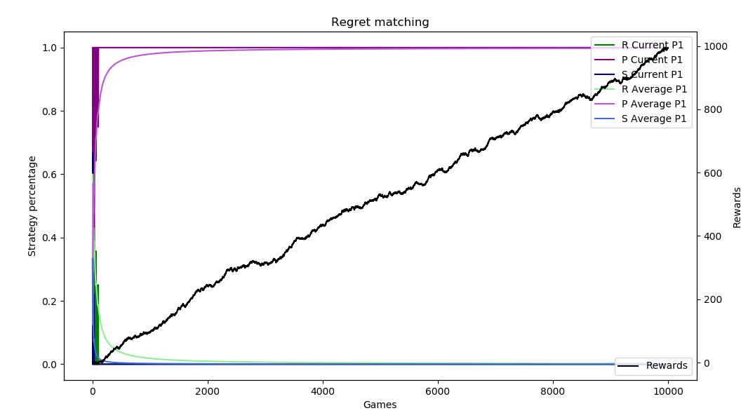
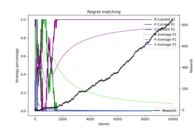
Depending on the run and how the regrets accumulate, the regret matching can figure this out immediately or it can take some time. Here are 10,000 sample runs of this scenario.
The plots show the current strategy and average strategy over time of each of rock (green), paper (purple), and scissors (blue). These are on a 0 to 1 scale on the left axis. The black line measures the profit (aka rewards) on the right axis. The horizontal axis is the number of sample runs. The top plot shows how the algorithm can sometimes “catch on” very fast and almost immediately switch to always playing paper, while the second shows it taking about 1,500 games to figure that out.
Regret in Poker
The regret matching method is at the core of selecting actions in the algorithms used to solve poker games. We will go into more detail in the CFR Algorithm section. In brief, each unique state of the game has a regret counter for each action and so the strategy is determined at each game state by using regret matching as the regrets get updated.